Introduction

Most people likely have experience with pivot tables in Excel. Pandas provides a similar function called pivot_table . While it is exceedingly useful, I frequently find myself struggling to remember how to use the syntax to format the output for my needs. This blog will focus on explaining the pandas pivot_table function and how to use it for your data analysis.

 

Objectives

• Introducing our data set
• Merge the data in a unique Dataframe
• Categorizing the data
• Creating a multi-index pivot table
• Visualizing the pivot table using plot()
• Manipulating the data using aggfunc
• Applying a custom function to remove outliers
• Categorizing using string manipulation
• Handling missing data
• Conclusion

 

Introducing our data set

Content

You are provided with historical sales data for 45 stores located in different regions - each store contains a number of departments. The company also runs several promotional markdown events throughout the year. These markdowns precede prominent holidays, the four largest of which are the Super Bowl, Labor Day, Thanksgiving, and Christmas. The weeks including these holidays are weighted five times higher in the evaluation than non-holiday weeks.

Within the Excel Sheet, there are 3 Tabs – Stores, Features and Sales

Stores

Anonymized information about the 45 stores, indicating the type and size of store

Features

Contains additional data related to the store, department, and regional activity for the given dates.

1. Store - the store number
2. Date - the week
3. Temperature - average temperature in the region
4. Fuel_Price - cost of fuel in the region
5. MarkDown1-5 - anonymized data related to promotional markdowns. MarkDown data is only available after Nov 2011, and is not available for all stores all the time. Any missing value is marked with an NA
6. CPI - the consumer price index
7. Unemployment - the unemployment rate
8. IsHoliday - whether the week is a special holiday week

Sales

Historical sales data, which covers to 2010-02-05 to 2012-11-01. Within this tab you will find the following fields:

1. Store - the store number
2. Dept - the department number
3. Date - the week
4. Weekly_Sales - sales for the given department in the given store
5. IsHoliday - whether the week is a special holiday week

 

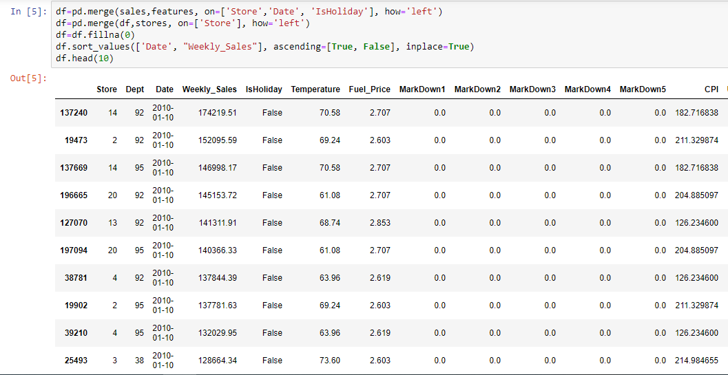
Merge the data in a unique DataFrame

 

Categorizing the data

 

The fun thing about pandas pivot_table is you can get another point of view on your data with only one line of code. Most of the pivot_table parameters use default values, so the only mandatory parameters you must add are data and index.

Though it isn’t mandatory, we’ll also use the value parameter in the next example.

1. data is self explanatory – it’s the DataFrame you’d like to use

2. index is the column, grouper, array (or list of the previous) you’d like to group your data by. It will be displayed in the index column (or columns, if you’re passing in a list)

3. values (optional) is the column you’d like to aggregate. If you do not specify this then the function will aggregate all numeric columns.

Let’s first look at the output, and then explain how the table was produced:

 

 

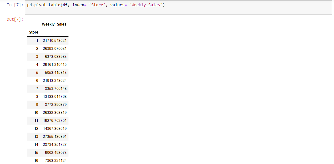
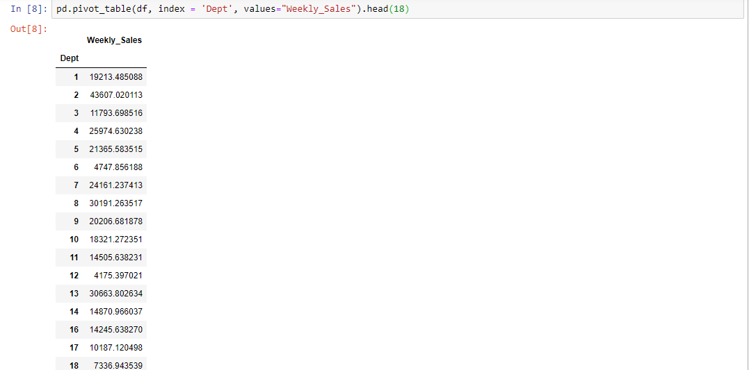
By passing Store as the index parameter, we chose to group our data by Store. The output is a pivot table that displays the 45 different values for Store as index, and the Weekly Sales as values. It’s worth noting that the aggregation default value is mean (or average), so the values displayed in the Weekly Sales column are the Store's average.

Next, let’s use the Dept column as index:

 

 

 

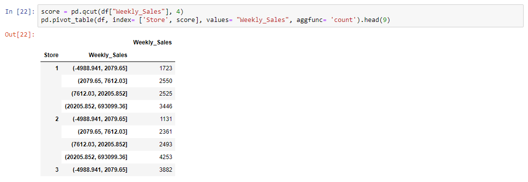
Creating a multi-index pivot table

 

The pivot_table() built-in function offers straightforward parameter names and default values that can help simplify complex procedures like multi-indexing.

In order to group the data by more than one column, all we have to do is pass in a list of column names. Let’s categorize the data by Dept and Date:

 

 

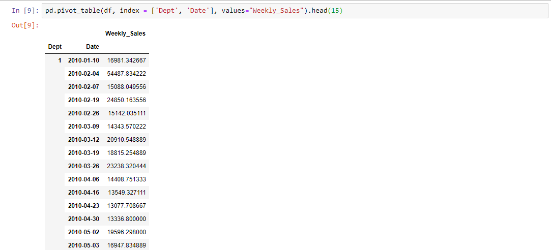
These examples also reveal where pivot table got its name from: it allows you to rotate or pivot the summary table, and this rotation gives us a different perspective of the data. A perspective that can very well help you quickly gain valuable insights.

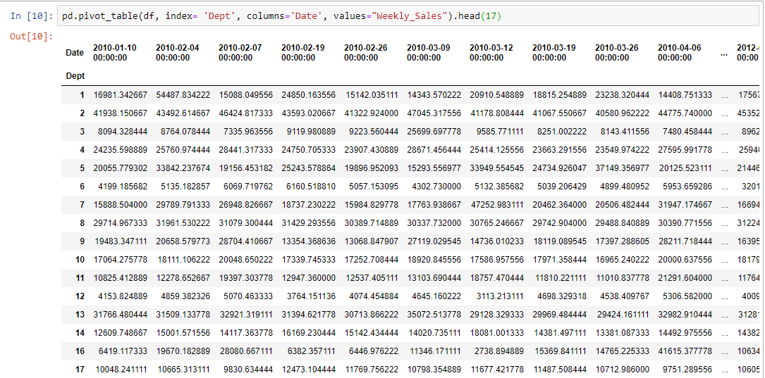
This is one way to look at the data, but we can use the columns parameter to get a better display:

columns is the column, grouper, array, or list of the previous you’d like to group your data by. Using it will spread the different values horizontally.

Using Date as the Columns argument will display the different values, and will make for a much better display, like so:

 

 

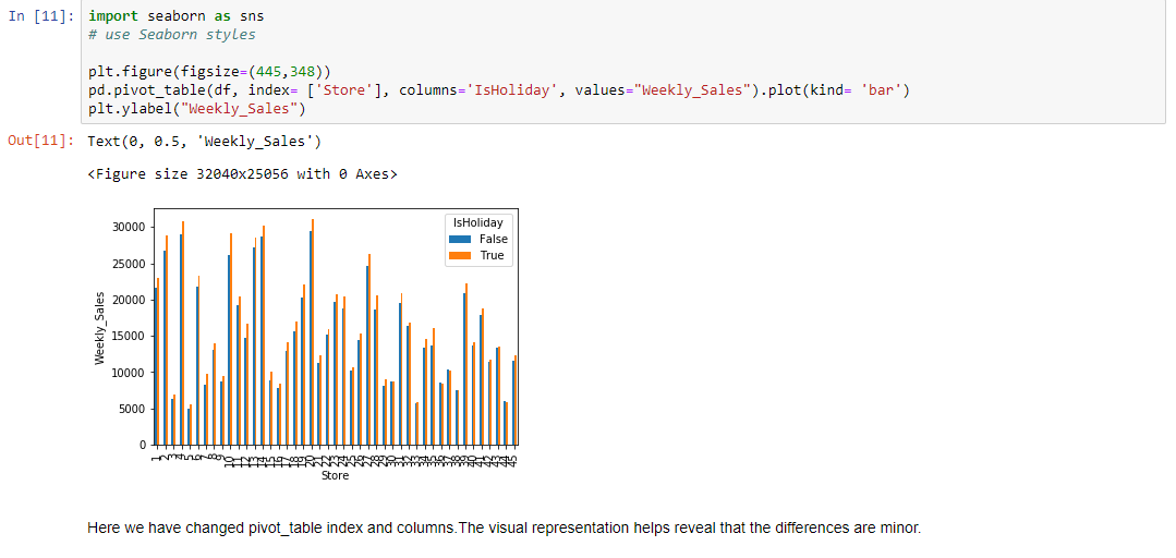
Visualizing the pivot table using plot()

 

Let's see the visual representation.

 

 

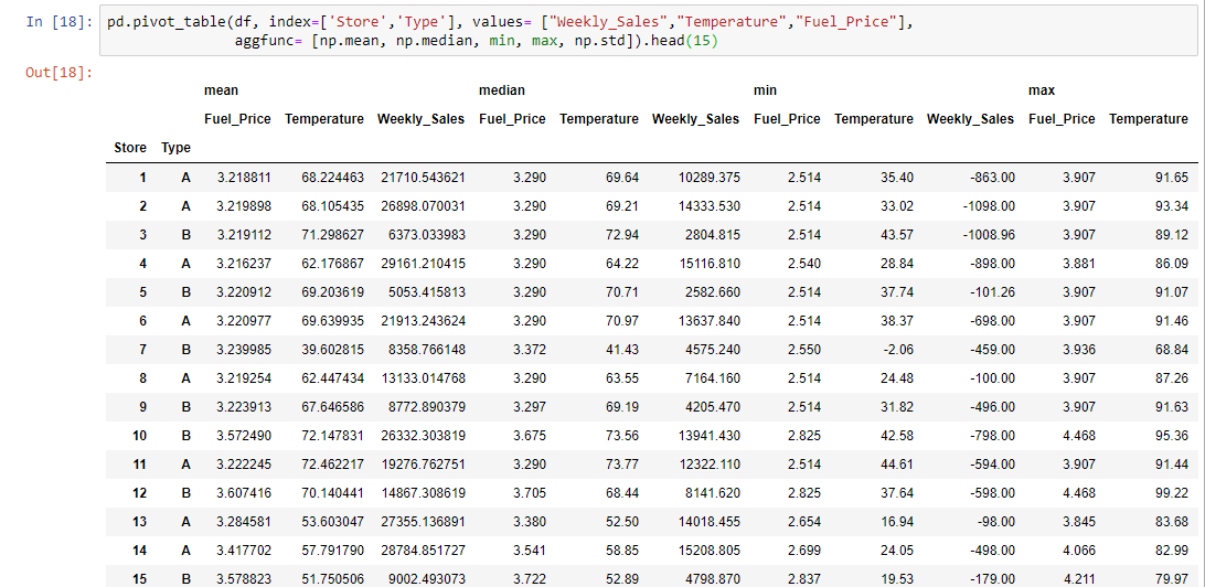
Manipulating the data using aggfunc

 

Up until now we’ve used the average to get insights about the data, but there are other important values to consider. Time to experiment with the aggfunc parameter:

• aggfunc (optional) accepts a function or list of functions you’d like to use on your group (default: numpy.mean). If a list of functions is passed, the resulting pivot table will have hierarchical columns whose top level are the function names.

Let’s add the median, minimum, maximum, and the standard deviation for each region. This can help us evaluate how accurate the average is, and if it’s really representative of the real picture.

 

 

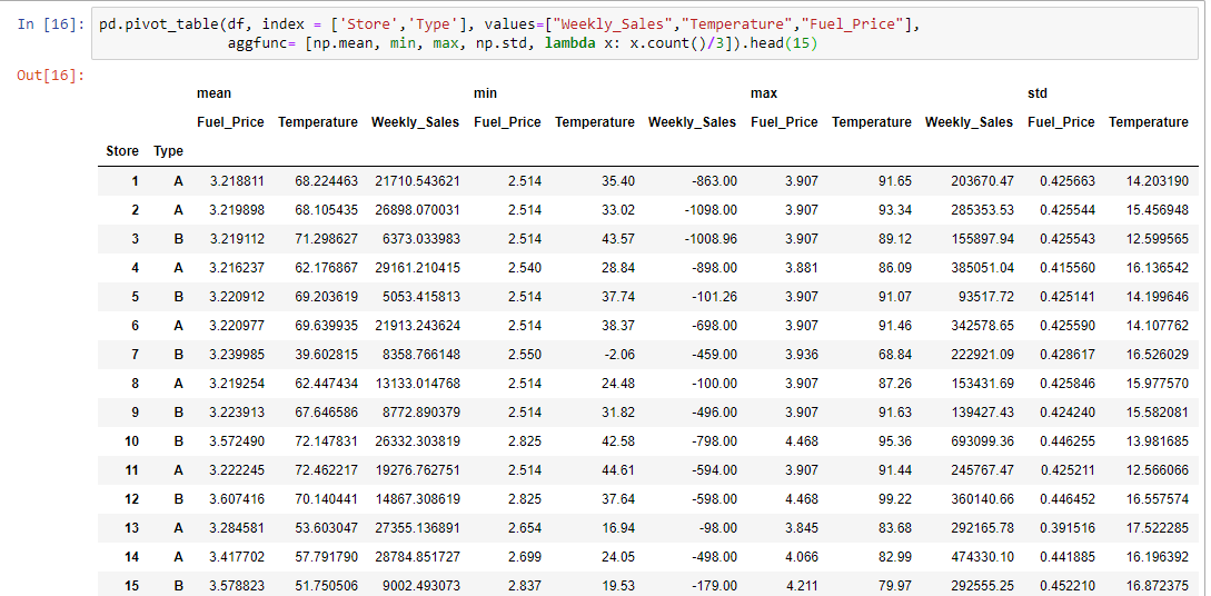
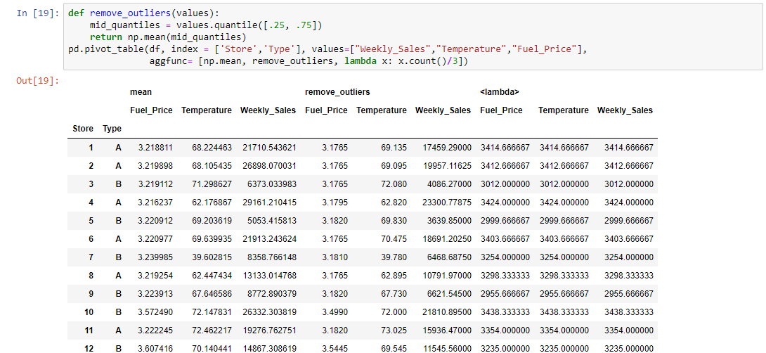
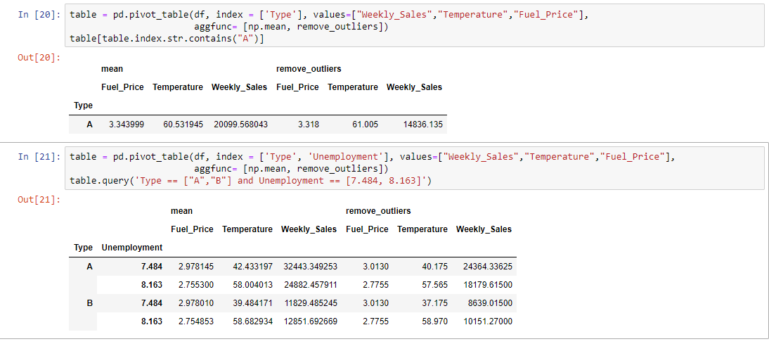
Applying a custom function to remove outliers

 

pivot_table allows you to pass your own custom aggregation functions as arguments. You can either use a lambda function, or create a function. Let’s calculate the average number of countries in each region in a given year. We can do this easily using a lambda function, like so:

 

 

Categorizing using string manipulation

 

 

Handling missing data

 

We’ve covered the most powerful parameters of pivot_table thus far, so you can already get a lot out of it if you go experiment using this method on your own project. Having said that, it’s useful to quickly go through the remaining parameters (which are all optional and have default values). The first thing to talk about is missing values.

1. dropna is type boolean, and used to indicate you do not want to include columns whose entries are all NaN (default: True)

2. fill_value is type scalar, and used to choose a value to replace missing values (default: None).

We don’t have any columns where all entries are NaN, but it’s worth knowing that if we did pivot_table would drop them by default according to dropna definition.

We have been letting pivot_table treat our NaN‘s according to the default settings. The fill_value default value is None so this means we didn’t replace missing values in our Data set. To demonstrate this we’ll need to produce a pivot table with NaN values.

 

 

Conclusion

 

If you’re looking for a way to inspect your data from a different perspective then pivot_table is the answer. It’s easy to use, it’s useful for both numeric and categorical values, and it can get you results in one line of code.